Optimizing Rabin-Karp Hashing

Intro

Daniel Lemire is a professor of computer science at TÉLUQ, who specializes in performance engineering. He is also a prolific blogger, and his posts are occasionally featured on Hacker News. If you somehow found your way to this blog, you are likely familiar with his writing. A few weeks ago, he posed the following question: “How fast is rolling Rabin-Karp hashing?”, for example as might be used in the Rabin-Karp string search algorithm.

A friend and I had some extra time over the past couple of days, and we figured it would be fun to explore the problem. As it turns out, the algorithm is a good way to build an understanding for low-level performance optimizations, in particular the role of dependency chain latency.

If you haven’t read Lemire’s post yet, I would suggest at least giving it a quick glance.

Notes

I should point out a few things about the benchmarking code provided by Lemire, that you might find useful if you decide to experiment yourself:

1. The choice of window sizes does not reflect any real world scenario (if the target string is 8 bytes, we can just load and compare the whole string in a normal register). In our benchmarks we used much larger values.

2. The reported throughput is the maximum recorded throughput per run. This isn’t necessarily a bad choice, but it can make the result a bit unstable. We changed that to reflect the average throughput over all runs. No results were substantially affected by this change.

3. The choice of \(31\) as the default evaluation point for the polynomial means that if the method gets inlined, and your compiler is aggressive enough (as clang is), you can end up with a highly specialized and very fast implementation being emitted that elides the multiplications (x*31 => (x << 5) - x), and which will confound all of your benchmarks. Lemire seems to be aware of this, and has __attribute__(noinline)everywhere. If you want to add methods to experiment with using his test harness, you’ll want to make sure to add that attribute to those methods.

4. I have tried to stay aligned with the conventions and naming from Lemire’s code. This may lead to some strange-looking style mismatches in the code.

Notation and Setup

To stay aligned with Lemire’s benchmarks, we will reuse the signature from his code:

size_t count_hits(
    const char *data,
    size_t input_length,
    size_t window_length,
    uint32_t B,
    uint32_t target
);

This counts the number of substrings of window_lengthwithin the input string that match the target hashcode. While it is not a particularly useful method, it does force us to compute and use the hashes.

For reference, all benchmarks were run on a Intel Xeon Platinum 8481C CPU (Sapphire Rapids).

Naive Approach

I won’t dwell on the naive approach too much, except to introduce the notation we’ll use throughout:

• The length of the input to be searched is \(n\). In the source code, we use the variable len to represent this.

• The window length, \(w\), is the length of the target string. Somewhat confusingly, in much of the source code, we use the variable N to represent this (this is from the original benchmark code).

• The input data array will either be referred to as data or as a. The latter comes from thinking of the input as an array \([a_0,a_1,...,a_{n-1}]\), or from the hash code as the series, for example \(a_0+a_1B+a_2B^2+...+a_{w-1}B^{w-1}\).

• The base is \(B\).

The naive approach takes time \(O(nw)\). We can’t even really benchmark it, as it very quickly becomes intractable to run.

Simple Rolling Approach

Again, I won’t dwell on this too much, except to paste the reference code, and establish a baseline benchmark. I’ll also point out that this algorithm is asymptotically optimal (requiring only a constant amount of work per input item), and uses O(w) memory.

Here’s the code from Lemire’s post:

__attribute__ ((noinline))
size_t karprabin_rolling(const char *data, size_t len, size_t N, uint32_t B, uint32_t target) {
    size_t counter = 0;
    uint32_t BtoN = 1;
    for (size_t i = 0; i < N; i++) {
        BtoN *= B;
    }
    uint32_t hash = 0;
    for (size_t i = 0; i < N; i++) {
        hash = hash * B + data[i];
    }
    if (hash == target) {
        counter++;
    }
    for (size_t i = N; i < len; i++) {
        hash = hash * B + data[i] - BtoN * data[i - N];
        if (hash == target) {
            counter++;
        }
    }
    return counter;
}

This runs at 0.73 GB/s.

Thinking about performance

Tools like perf are great. But in my experience, it’s useful to try to form a hypothesis before breaking out a profiler. This helps ground the process, and forces us to develop and update a mental model of the performance of the code as we investigate. I’ve also found this general approach to be useful at other scales (for example when analyzing bottlenecks in distributed systems).

A good starting point is to be able to bound the problem in some way. So with that in mind, let’s throw together a quick benchmark for computing the simpler hash function, that’s just a sum of the values over the sliding window (you could think of this as a Rabin-Karp hash with \(B=1\)):

__attribute__ ((noinline))
size_t sum_rolling(const char *data, size_t len, size_t N, uint32_t B, uint32_t target) {
    size_t counter = 0;

    uint32_t hash = 0;
    for (size_t i = 0; i < N; i++) {
        hash = hash + data[i];
    }
    if (hash == target) {
        counter++;
    }
    for (size_t i = N; i < len; i++) {
        hash = hash + data[i] - data[i - N];
        if (hash == target) {
            counter++;
        }
    }
    return counter;
}

This runs at 1.49 GB/s.

Returning to our actual problem, let’s try to build an intuition for where the opportunities to optimize lie. Consider the instructions that are executed on each loop iteration:

1. Load two values (the incoming and outgoing elements).

2. Multiply the outgoing element by \(B^n\).

3. Multiply the hash by \(B\).

4. Add the incoming element and subtract the (scaled) outgoing element to the hash.

5. Do some bounds checking, update loop variables, etc..

On one hand, this seems pretty good. Multiplication on Sapphire Rapids has a latency of 4 cycles. This core is clocked (when boosted) at 3.8GHz, so this implementation is processing one item every 5 ticks. We could try to squeeze out a little bit more performance by manually unrolling the loop (as Lemire does in his reference code). In our case, that doesn’t make any difference, because the compiler has already helpfully unrolled the loop for us.

The bigger issue is that we have a lot of idle silicon sitting around. And the cause of this is the dependency chain between the hash code computations. For example, the first three hashes are:

We clearly cannot start to compute \(H_2\) before we have computed \(H_1\), and so must wait to issue the multiplication \(B*H_1\) until we have computed \(H_1\), which involves computing \(B*H_0\), which takes at least 4 cycles. This is what’s known as a loop-carried dependency. The processor can try to stay busy by executing the other operations while the multiply is running, but ultimately the latency of the multiplication puts a limit on the overall throughput.

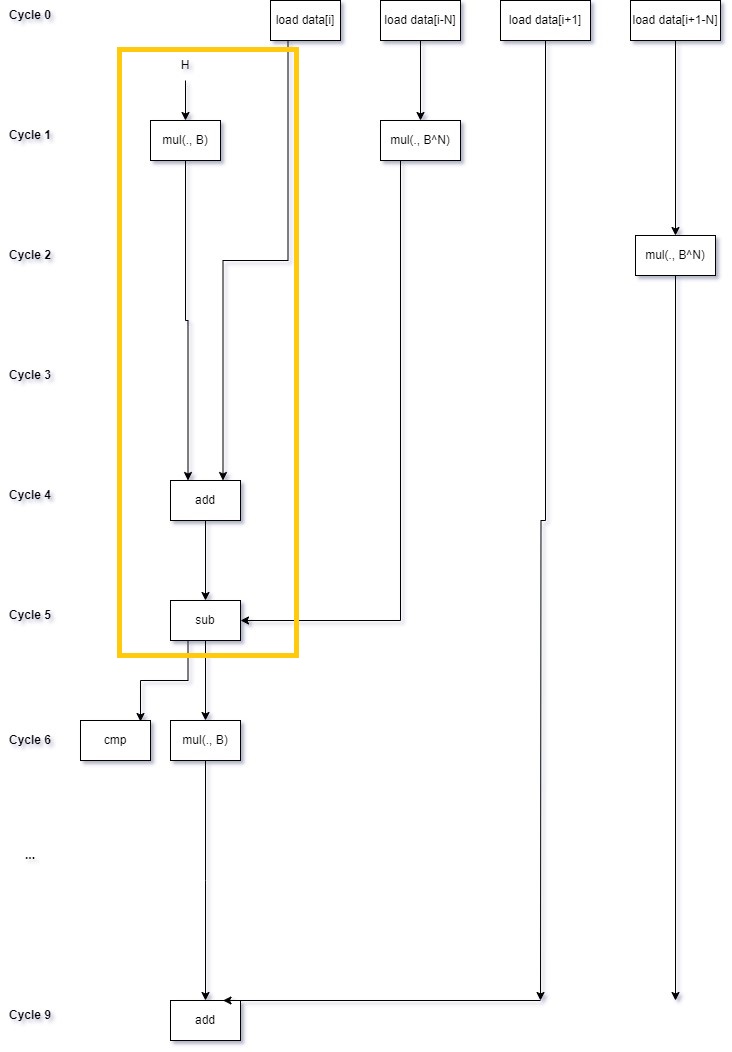
To see this, I find it helpful to draw out the computation graph over time (here is a very good overview of the general technique). Time flows downward, and arrows represent data dependencies between instructions. I’ve drawn out part of an iteration of an unrolled loop (I only included the loads for two windows to avoid cluttering things up too much). I’ve also highlighted the loop-carried dependency:

This may not line up exactly with the exact instructions that the processor executes in parallel, but does give the gist of it. Of particular note, you can see that the multiplications of the elements falling out of the window can be issued long before they are needed. It’s the dependency on multiplying the hash by \(B\) is the bottleneck.

“Parallelizing” the Process

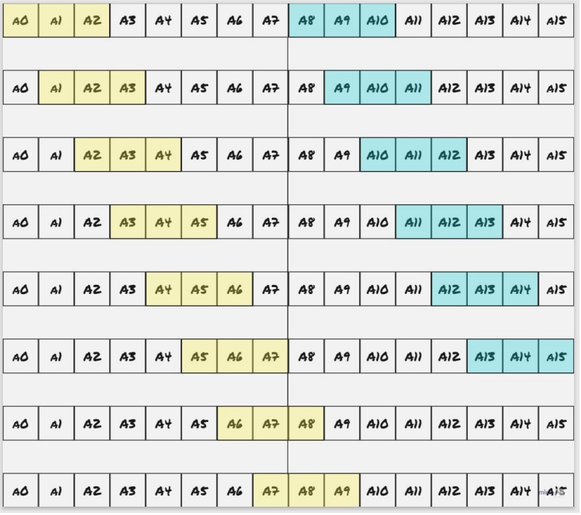
One approach to getting around the chain dependency would be to simply split the input in half, and process each half in its own thread. Note that you have to do a little redundant work here. If we decide on the convention that each thread processes all hashes that begin within its half of the data, then the first thread needs to process an extra window’s worth of values.

Here’s an example of what the process might look like with a window of size 8:

In practice, the input length is much larger than the target window size, so this is not a very high cost to pay.

Spinning up a thread pool doesn’t seem in keeping with the spirit of the exercise. But as we just discovered, even a single core has plenty of extra capacity. So if we just simply issue the two hash code computations in a single thread, we should still be able to take advantage of all of the OOO-superscalar features of modern processors. And indeed we see a dramatic speedup.

This runs at 1.25 GB/s.

How far can we push this approach? At least on our test host, doubling from 2 independent hash codes to 4 yielded no benefits, but YMMV.

Making it Streaming Friendly

Processing the data in this way introduces a very big shortcoming: the algorithm can no longer be applied to a single stream (because we need to be able to seek halfway through the input). I can imagine plenty of use cases where that would be a dealbreaker. How can we get that behavior back? The best approach I can think of is to read a fairly large chunk of data, say some constant \(C\) windows’ worth, for \(C\) around 10 or so. Then process that chunk in “parallel” as described above. Then read and process the next chunk. Now, instead of processing an extra window once, we process two extra windows per chunk (one in the middle and one at the end), and we have to hold \(C\) windows in memory. So the memory consumption is \(O(C*W)\), and the runtime is \(O(N*(1+\frac{2}{c}))\). By playing with the constant \(C\), we can trade off memory consumption and runtime overhead. We get back a streaming-friendly algorithm, which I call the chunked streaming algorithm, and the performance doesn’t suffer too much. For \(C=32\), we can process the input at 1.20 GB/s.

SIMD

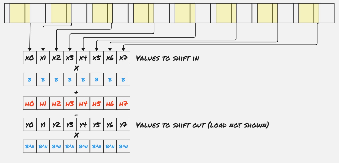
One nice feature of this approach is that is very easily adapted to the Intel AVX2 instructions. Instead of splitting each chunk into 2 parts, we can split each chunk into 8 parts, which I’ll call “slices” (each AVX2 register consists of 8 32-bit values), and process each part independently within a single 32-bit slice.

Note that in the code below, in each loop iteration we read 4 values per slice (so 32 in total), and explicitly unroll the loop. This lets us issue only two gathers per iteration, which is a big savings.

static inline __m256i constant_ymm(uint32_t x) {
    return _mm256_set_epi32(x, x, x, x, x, x, x, x);
}

// Byte extractors

static inline __m256i byte0(__m256i bytes) {
    return _mm256_srai_epi32(_mm256_slli_epi32(bytes, 24), 24);
}

static inline __m256i byte1(__m256i bytes) {
    return _mm256_srai_epi32(_mm256_slli_epi32(bytes, 16), 24);
}

static inline __m256i byte2(__m256i bytes) {
    return _mm256_srai_epi32(_mm256_slli_epi32(bytes, 8), 24);
}

static inline __m256i byte3(__m256i bytes) {
    return _mm256_srai_epi32(bytes, 24);
}

__attribute__ ((noinline))
size_t karprabin_rolling4_chunked_streaming_8x4_avx2(const char *data, size_t len, size_t N, uint32_t B, uint32_t target) {
    uint32_t BtoN = 1;
    for (size_t i = 0; i < N; i++) {
        BtoN *= B;
    }

    size_t counter = 0;

    size_t subblock_size = 4 * N;
    size_t block_size = 8 * subblock_size;

    __m256i targets = constant_ymm(target);
    __m256i bs = constant_ymm(B);
    __m256i bns = constant_ymm(BtoN);
    __m256i offsets = _mm256_set_epi32(
        7 * subblock_size,
        6 * subblock_size,
        5 * subblock_size,
        4 * subblock_size,
        3 * subblock_size,
        2 * subblock_size,
        subblock_size,
        0
    );

    __m256i hashes = _mm256_setzero_si256();
    const char* block_start = data;
    while ((block_start - data) + block_size + N < len) {
        // Initialize hashes
        hashes = _mm256_setzero_si256();

        for (size_t i = 0; i < N; i++) {
            __m256i as = _mm256_srai_epi32(
                _mm256_slli_epi32(
                    _mm256_i32gather_epi32((const int *) (block_start + i), offsets, 1),
                    24
                ),
                24
            );
            hashes = _mm256_add_epi32(
                _mm256_mullo_epi32(hashes, bs),
                as
            );
        }

        uint32_t first = _mm256_extract_epi32(hashes, 0);
        if (first == target) {
            counter++;
        }

        for (size_t i = 0; i < subblock_size; i+=4) {
            // Values to be added in
            __m256i as = _mm256_i32gather_epi32(
                (const int*) (block_start + i + N),
                offsets,
                1
            );
            // Values to be dropped off
            __m256i ans = _mm256_i32gather_epi32(
                (const int*) (block_start + i),
                offsets,
                1
            );

            // Value 0
            hashes = _mm256_sub_epi32(
                _mm256_add_epi32(
                    _mm256_mullo_epi32(hashes, bs),
                    byte0(as)
                ),
                _mm256_mullo_epi32(byte0(ans), bns)
            );
            counter += __builtin_popcount(_mm256_cmpeq_epi32_mask(hashes, targets));

            // Value 1
            hashes = _mm256_sub_epi32(
                _mm256_add_epi32(
                    _mm256_mullo_epi32(hashes, bs),
                    byte1(as)
                ),
                _mm256_mullo_epi32(byte1(ans), bns)
            );
            counter += __builtin_popcount(_mm256_cmpeq_epi32_mask(hashes, targets));

            // Value 2
            hashes = _mm256_sub_epi32(
                _mm256_add_epi32(
                    _mm256_mullo_epi32(hashes, bs),
                    byte2(as)
                ),
                _mm256_mullo_epi32(byte2(ans), bns)
            );
            counter += __builtin_popcount(_mm256_cmpeq_epi32_mask(hashes, targets));

            // Value 3
            hashes = _mm256_sub_epi32(
                _mm256_add_epi32(
                    _mm256_mullo_epi32(hashes, bs),
                    byte3(as)
                ),
                _mm256_mullo_epi32(byte3(ans), bns)
            );
            counter += __builtin_popcount(_mm256_cmpeq_epi32_mask(hashes, targets));
        }

        block_start += block_size + 1;
    }

    // Deal with what's left over
    size_t last_end = (block_start - data) + N - 1;
    uint32_t hash = _mm256_extract_epi32(hashes, 7);
    for (size_t i = last_end; i < len; i++) {
        hash = hash * B + data[i] - BtoN * data[i - N];
        if (hash == target) {
            counter++;
        }
    }

    return counter;
}

This runs at 1.59 GB/s.

Optimizing Further

The SIMD operations make things much faster, but frustratingly, we are again bound on the chain dependency between multiplying the hashcodes by \(B\). In some sense, we are a victim of our success here. By combining the separate multiplications into a single instruction, we freed up formerly occupied execution ports. But it would be nice to remove this bottleneck. One approach (which I have not tried) is to do the same trick as before, and process two of these parts in parallel.

Another (which we will go with) is to notice that while the multiplication instruction (vpmulld) has a latency of 10 cycles, the processor can issue that instruction every 0.66 cycles. Put another way, issuing a bunch of SIMD multiplications in a row is not much more expensive than issuing a single one.

Recasting the problem

To take advantage of this fact, let’s recast the problem slightly. In our current implementation, we compute the hash over each window and then compare it to the target:

We did this because it makes the recurrance very straightforward to calculate. But we could just as easily have reversed things:

Assuming that \(B\) is odd, we can compute the multiplicative inverse \(B^{-1}\), and compute the hash with the recurrance:

We still need to multiply that hash in each loop iteration. What would happen if we did not scale them in each loop iteration?

This is just the result of taking rolling sums of the power series:

At first, this may not seem particularly useful, but it’s easy to see that the new hash \(H'\) and old hash \(H\) are related by:

And thus:

So to determine if the hash matches the target, we just need to scale the target by \(B^n\), before comparing them.

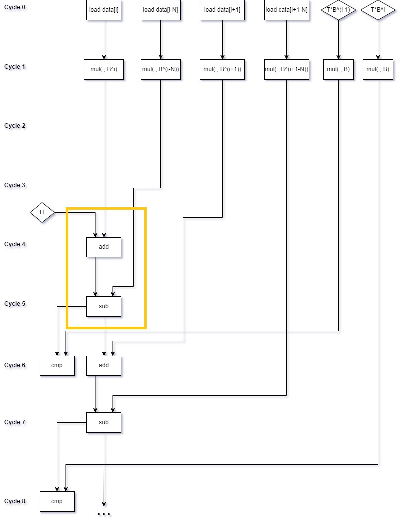
Why is this an improvment? While we (paradoxically) actually have to compute more multiplications, we have gained something, namely that the multiplications can now all be issued at the same time. To illustrate this, let’s consider the non-SIMD case. I’ve grouped instructions at the earliest cycle where they could execute. In practice, they will probably execute later, when an execution port becomes available. Values in registers are represented by diamonds. As before, I’ve highlighted the chain dependency:

We can see that the chain dependency has gone from a multiplication, addition and subtraction to just an addition and subtraction. All of the multiplications can be issued at the beginning of the loop iteration.

This runs at 1.77 GB/s.

Here’s what a non-SIMD version of this approach might look like. To see how the multiplications can be issued at once, I’ve explicitly unrolled the loop (just to a factor of 2):

__attribute__ ((noinline))
size_t karprabin_rolling2_alternate(const char *data, size_t len, size_t N, uint32_t B, uint32_t target) {
    size_t counter = 0;
    uint32_t B2 = B*B;
    uint32_t BtoN = 1;
    for (size_t i = 0; i < N; i++) {
        BtoN *= B;
    }

    uint32_t hash = 0;
    for (size_t i = 0; i < N; i++) {
        hash = hash * B + data[i];
    }
    // This is always equal to B^i
    uint32_t shift_in0 = 1;
    // This is always equal to B^(i+1)
    uint32_t shift_in1 = shiftin_0 * b;
    // This is always equal to B^(i-N)
    uint32_t shift_out0 = 1;
    // This is always equal to B^(i-N+1)
    uint32_t shift_out1 = B;
    // This is always equal to target * B^(i-N)
    uint32_t target0 = target;
    // This is always equal to target * B^(i-N+1)
    uint32_t target1 = target * B;

    if (hash == target) {
        counter++;
    }
    size_t i = N;
    for (; i + 1 < len; i += 2) {

        hash = hash + shift_in0 * data[i] - shift_out0 * data[i - N];
        if (hash == target0) {
            counter++;
        }
        hash = hash + shift_in1 * data[i+1] - shift_out1 * data[i - N + 1];
        if (hash == target1) {
            counter++;
        }

        // Update the shift factors and targets
        // They are multiplied by B^2 because the loop is unrolled with a factor of 2
        // Note that all of these instructions can be issued at once
        shift_in0 *= B2;
        shift_in1 *= B2;
        shift_out0 *= B2;
        shift_out1 *= B2;
        target0 *= B2;
        target1 *= B2;
    }

    // ...
    // Deal with any remaining elements
    // ...

    return counter;
}

A final optimization

There’s one more optimization I’d like to discuss. I don’t really like it, because it makes the method much less useful, but we can do a bit better at counting the number of matches. Instead of counting up hash matches in a single accumulator, we can keep track of the number of matches in each “slice”, and then sum them up at the end. That is, replace:

size_t counter = 0;
// ...
counter += __builtin_popcount(_mm256_cmpeq_epi32_mask(hashes, targets));
// ...
return counter;

with:

__m256i counts = _mm256_setzero_si256();
// ...
matches = _mm256_srli_epi32(_mm256_cmpeq_epi32(hashes, targets), 31);
counts = _mm256_add_epi32(counts, matches);
// ...
return _mm256_extract_epi32(counts, 0)
    + _mm256_extract_epi32(counts, 1)
    + ...;

_mm256_cmpeq_epi32 fills the corresponding 32-bit value with 0xFFFFFFFF if the values match, so shifting by 31 will result in a 1 in the slice if the hash matches the target.

The reason I don’t like this is that while _mm256_cmpeq_epi32_mask produces an output that can be used for actual string search, I cannot think of a good use case for simply counting the number of hash matches. But it was an interesting optimization, so I left it in.

This runs at 1.86 GB/s.

Update: A commenter on HackerNews points out that 0xFFFFFFFF is just -1 in two’s complement arithmetic, there’s no need to shift. Instead, just do this:

__m256i counts = _mm256_setzero_si256();
// ...
matches = mm256_cmpeq_epi32(hashes, targets);
counts = _mm256_sub_epi32(counts, matches);
// ...
return _mm256_extract_epi32(counts, 0)
    + _mm256_extract_epi32(counts, 1)
    + ...;

This yields a modest improvement, to 1.89 GB/s.

Summary

All in all, we were able to achieve a greater than 2.5x speedup. It was interesting to poke around the AVX instructions after a while away from them, and I definitely feel like I have a better intuition for these kinds of problems after working through this. Thanks to Daniel Lemire for posing the problem and providing his benchmark harness.

The Elementary (Fast) Fourier Transform

In math curricula, the Fast Fourier Transform is usually encountered in fairly advanced classes. For example, you might first come across it in a course on Real Analysis or Digital Signal Processing. My own undergraduate math courses started with Fourier series, then moved on to the (continuous) Fourier transform, then the discrete-time Fourier transform and discrete Fourier transform. The FFT is introduced as more of a corollary optimization. In engineering courses, it comes up all the time, but almost always as a tool to move between the time domain and frequency domain, to the point where the Fast Fourier Transform (which is an algorithm) becomes a synecdoche for the transform itself.

This is a shame, because the FFT does not use any advanced mathematics, requiring only an understanding of the algebra of complex numbers. Here I try to explain it in such a way. As we go, I will add some snippets of Python code, eventually building up to a complete implementation.

After writing this, I found that there is a pretty good overview at 3Blue1Brown, that largely follows along the same lines. I hope this fleshes out some of the detail that the video glosses over.

Motivation: (Fast) Convolutions

Instead of starting with the Fourier Transform, let’s start with a related transform: the discrete convolution (from now on, everything will be implicitly discrete). In fact, let’s start at an even higher level: the digital filter.

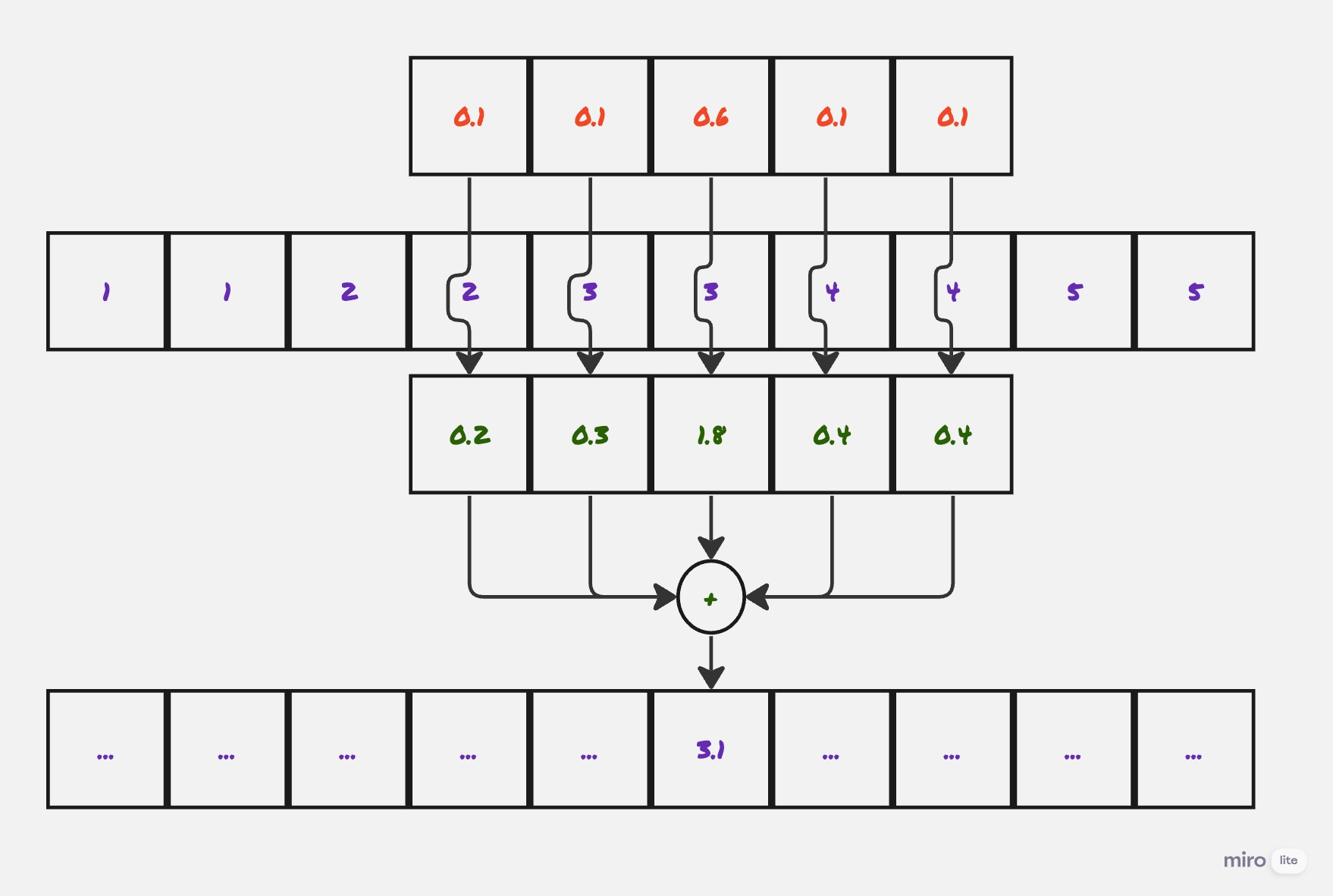
Suppose you have recorded \(N\) samples of audio at some frequency, call it \(A=A[0..N-1]\). The audio quality might be absolutely pristine, but more likely it’s been corrupted by glitches, noise, wind, pops and clicks from people bumping into the microphone, and so on. What can we do to clean up the signal? One common approach, at least for phenomena that are of short duration (such as pops and clicks) is to filter it. For example, we might replace each sample of the signal with the moving average of the \(5\) values before and the \(5\) values after it. Or we might want to use a more elaborate filter with a larger support, such as a Gaussian.

The way I think about this operation is that the filter slides along the signal. And at each stage, you perform a pointwise multiplication of the filter and the overlapping region of the signal, and sum up the values (mathematically this is just an inner product).

Mathematically, if you have a signal \(A[0..N]\) and a kernel \(B[0..M]\), for odd \(M\) (so that the sum below is balanced), then the convolution is:

(Here follow the convention that if \(A[k]\) is zero for \(k < 0\) or \(k \ge |A|\).)

Another way to write this is to note that \((n-k) + k = n\), so:

This formulation will be more useful for us later. The smoothing function is typically referred to as the filter or as the kernel. This operation, of smoothing out one function by another, comes up all the time in math, signals analysis, and engineering, and is known as the convolution. To name but a few examples, it’s used to implement antialiasing filters in audio and graphics, to compute spectrograms in signals analysis, for edge detection in image analysis. It is also the central operation in the convolutional neural network. It’s definitely useful to be able to perform it quickly.

So, let’s start with a method declaration:

Signal = typing.NewType("Signal", numpy.ndarray)

def convolution(signal: Signal, filt: Signal) -> Signal:
    ...

Convolutions and Polynomial Multiplication

Convolutions are equivalent to polynomial multiplication

The thing is, everyone who has taken an Algebra II course has seen this operation before, just under a different name: polynomial multiplication. Given two polynomials:

Their product is given by:

Note that this is exactly equivalent to computing the convolution of the sequences \(A=[a_0,a_1,...,a_n]\) and \(B=[b_0,b_1,...,b_m]\).

That is, the coefficient of \(x^i\) in their product as polynomials is equal to the \(i^{th}\) value of their convolution as sequences. So we can restate our problem: Given two polynomials \(a(x)\) and \(b(x)\), compute (the coefficients of) their product \(a(x)b(x)\).

Let’s quickly think through the runtime complexity of this problem. By directly computing the product, multiplying each pair of coefficients in the two multiplicands, we can compute the product in time \(O(nm)\). But, as we will see, we can do better.

# A list of coefficients
PolyCoeffs = typing.NewType("PolyCoeffs", list[float])

def product_naive(a: PolyCoeffs, b: PolyCoeffs) -> PolyCoeffs:
    result = [0 for _ in range(len(a) + len(b))]
    for ai, ac in enumerate(a):
        for bi, bc in enumerate(b):
            result[ai+bi] += ac * bc
    return PolyCoeffs(result)

Representations of Polynomials

Why recast the convolution in this way? Because we can exploit our knowledge of polynomials, in particular, that polynomials can be represented in multiple ways. The usual way, as a list of coefficients, is one. Another common way is by a constant and its set of roots, as in \(f(x)=c(x-r_0)(x-r_1)...(x-r_n)\).

And, relevant to our use case, you can represent an \(n^{th}\) degree polynomial by its value on \(n+1\) distinct points (you end up with a system of \(n+1\) equations and \(n+1\) variables). Just to work through an example, suppose that you have a second degree polynomial (a quadratic) \(f(x)=2x^2+x+7\), and we choose to represent it by its values on \(\lbrace 0,1,2 \rbrace\):

Then we end up with the following system of equations:

Which we can solve in the usual way:

So, \(f(x) = 2x^2 + x^1 + 7x^0\), as expected. This representation is known as the point-value representation. From now, we will adopt the convention that lower-case letters refer to polynomials in their coefficient form, and upper-case letters refer to them in their point-value representations.

Here’s a type for a list of values, and for moving back and forth between the representations:

Values = typing.NewType("Values", list[complex])

class Representation(Protocol):
    def to_values(self, coeffs: PolyCoeffs) -> Values:
        ...

    def to_coeffs(self, values: Values) -> PolyCoeffs:
        ...

Why use point-value representation?

The point-value representation is a natural choice for our problem, because multiplication in this domain is very fast, just being the pointwise product of the values. Note that if \(a(x)\) has degree \(n\) and \(b(x)\) has degree \(m\), their product \(a(x)*b(x)\) will have degree \((n+m)\). So if you have evaluated \(a(x)\) and \(b(x)\) on a set of \((n+m+1)\) points, giving:

Then the representation of their product \(a(x)b(x)\) is:

This requires only \((n+m)\) multiplications to compute. Or in code:

def product_values(a: Values, b: Values) -> Values:
    return Values([ai * bi for ai, bi in zip(a, b)])

We can start to see the shape of a fast algorithm for polynomial multiplication (and thus convolutions). Given two polynomials, \(a(x)\) and \(b(x)\):

In code:

def product_faster(
        a: PolyCoeffs,
        b: PolyCoeffs,
        rep: Representation
) -> PolyCoeffs:
    # Convert to values
    av = rep.to_values(a)
    bv = rep.to_values(b)
    # Multiply pointwise
    prod = product_values(av, bv)
    # Convert back
    return rep.to_coeffs(prod)

At first, it does not seem like we have made our situation any better. For example, by using Horner’s method, step \((2)\) would take \(O((n+m)^2)\) time, no better than the naive method. We have not addressed step \((5)\) at all, and it is not obvious that we can perform steps \((2)\) and \((3)\) any faster than the naive multiplication algorithm.

Computing point-value representations

Not obvious, but true. There is in fact a set of points on which you can evaluate a polynomial quickly. This is the only part of the algorithm that requires even moderately advanced mathematics. Instead of just telling you, it’s worth thinking through how you might have thought it up.

Say you were approaching this problem for the first time. One thread to pull on is that evaluating polynomials has a recursive structure. Given a polynomial \(a(x)=a_0+a_1x^1+a_2x^2+...+a_nx^n\) of degree \(n\) (for now, say \(n\) is odd), we can split it into “even” and “odd” parts:

These two parts look like polynomials in \(x^2\), and indeed they are, of degree \({\lceil n/2 \rceil}\):

If you’ve studied algorithms at all, this might start to look like dynamic programming. We’ve split the problem into recursive subproblems. Now can we figure out how to reuse our work from those subproblems? This brings us to the main insight that makes the Fast Fourier Transform possible (and why the variable switched from \(\mathbf{x}\) to \(\mathbf{z}\)). There is a family of sets of points \(W_n\), for which \(z^2 \in W_{n/2} \ for \ all \ z \in W_n\), namely the \({n^{th}}\)complex roots of unity. If \(z\) is an \(n^{th}\) root of unity (say for even \(n\)), then we have, for some \(k\):

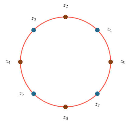
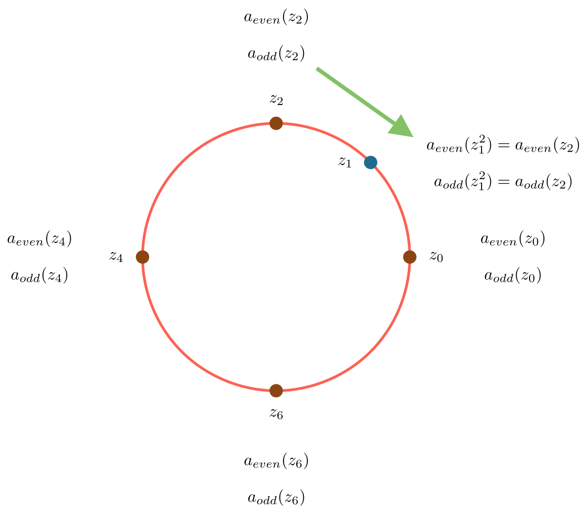
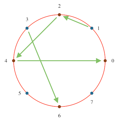
And we see that \(z^2\) is an \((n/2)^{th}\) complex root of unity. This can be a little tricky, so let’s draw it out for a specific example. Below, you can see the \(8^{th}\) roots of unity, labelled \(0\) to \(7\), so that the \(k^{th}\) root is equal to \(e^{2\pi i k/8}\). The \(4^{th}\) roots of unity are colored brown. The green arrows show the result of squaring each root (to keep the image from being too cluttered, I’ve only shown the first half). And you can see that, indeed, the square of each \(8^{th}\) root of unity is a \(4^{th}\) root of unity.

Why is this a big deal? Because we can reuse the work from the smaller subproblems in our recursive formulation. Say that we have computed \(a_{even}(z)\) and \(a_{odd}(z)\) on the complex \((n/2)^{th}\) roots of unity, and stored them in arrays \(A_{even}[0..n/2]\) and \(A_{odd}[0..n/2]\).

Given a complex \(n^{th}\) root of unity, \(z\), as we discussed earlier, \(z^2\) is an \((n/2)^{th}\) root of unity, and so we do not need to recompute \(a_{even}(z^2)\) and \(a_{odd}(z^2)\). We can just look them up in the arrays \(A_{even}\) and \(A_{odd}\). There is a lot of algebra here, which obscures what is actually a simple operation. I find pictures easier to understand.

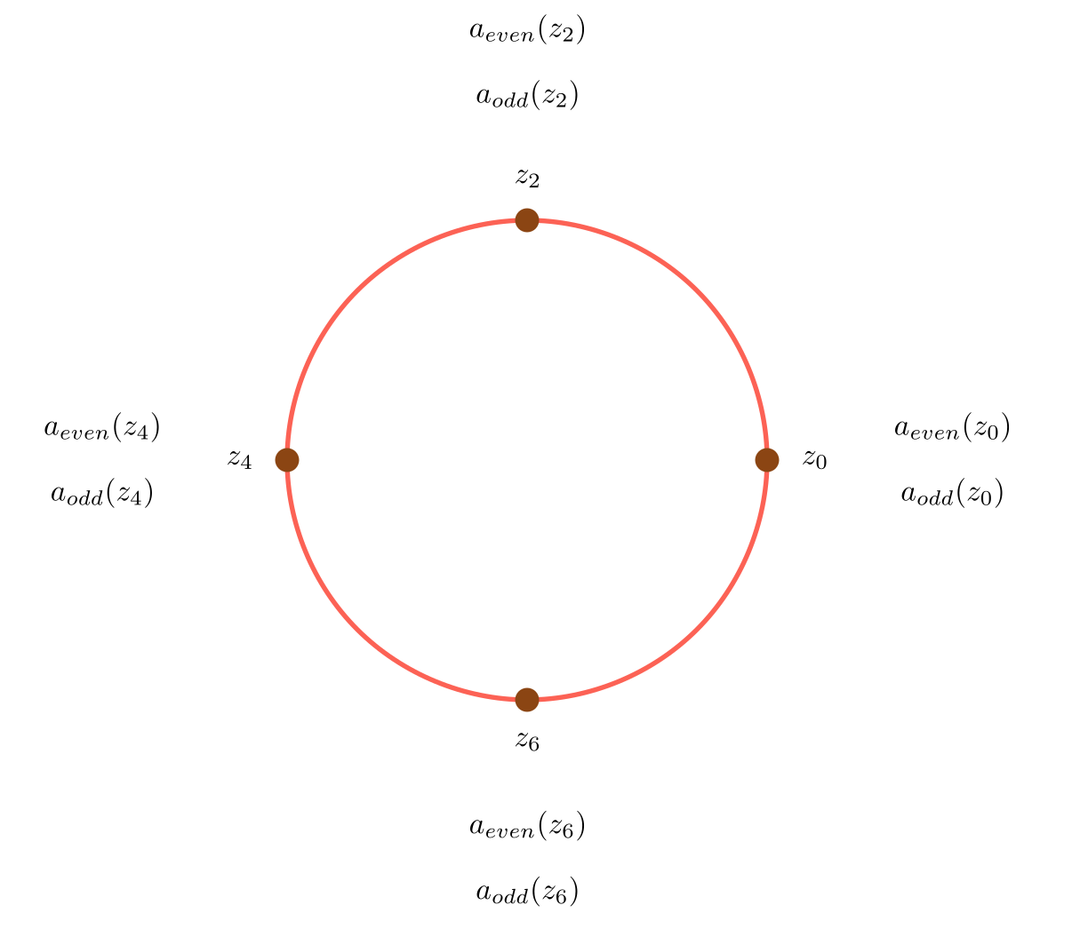
Say \(n=8\). Start with the \(n^{th}\) roots of unity:

Recursively compute \(A_{even}\) and \(A_{odd}\) on the \((n/2)^{th}\) roots of unity (every other point).

To compute, say \(a(z_1)\), we look up the values for \(a_{even}(z_2)\) and \(a_{odd}(z_2)\) (as \(z_1^2=z^2\)):

So the whole recursive algorithm is:

Step \((3)\) just requires two lookups, a single complex multiplication and a single complex addition.

Perhaps surprisingly, there isn’t much code. For now, let’s assume that \(n=2^m-1\) for some \(m\), so that the recursion is nice and simple. It won’t affect the asymptotic runtime, as you at most have to double the number of coefficients in the polynomial.

class RootsOfUnityRepresentation(Representation):
    """A degree n polynomial is represented by its value on the n^th roots of unity"""

    def to_values(self, coeffs: PolyCoeffs) -> Values:
        n = len(coeffs)
        if n == 1:
            # Polynomial is just a constant
            return Values([coeffs[0]])
        if (n & (n - 1)) != 0:
            raise ValueError("Expected a power of two sized input")
        # Split into a_even and a_odd, and recursively compute
        # even[k] is equal to a_even(z), for z = e^[(2πik/)(n/2)] = e^(4πik/n), the k^th, n/2^th-root of unity.
        even = self.to_values(PolyCoeffs([coeffs[i] for i in range(0, n, 2)]))
        odd = self.to_values(PolyCoeffs([coeffs[i] for i in range(1, n, 2)]))

        result = []
        for k in range(n):
            # Root is e^(2*pi*i/k)
            # Given n is always a power of two, this can be improved (for example by using the half-angle formula)
            root = complex(math.cos(2 * math.pi * k / n), math.sin(2 * math.pi * k / n))
            # If z = e^(2πik/n), then z^2 = e^(4πik/n) and:
            #   a_even(z^2) = even[k % (n/2)]
            #   a_odd(z^2) = odd[k % (n/2)]
            even_value = even[k % len(even)]
            odd_value = odd[k % len(odd)]
            # a(z) = a_even(z^2) + z*a_odd(z^2)
            result.append(even_value + root * odd_value)
        return Values(result)

By the way, this transformation, of representing a polynomial by its value on the roots of unity, has a name. It’s called the Discrete Fourier Transform. And this recursive implementation of it is known as the Fast Fourier Transform (specifically the Cooley-Tukey Algorithm). So if you’ve made it this far, congratulations. You now understand the FFT.

Runtime

What’s the runtime of this algorithm? Call it \(F(n)\), for a polynomial of degree \(n\). We have to:

1. Call the function recursively on \(a_{even}\). This takes time \(F(n/2)\).

2. Call the function recursively on \(a_{odd}\). This also takes time \(F(n/2)\).

3. For each of the \(n\) roots of unity, perform a (complex) multiplication and an addition. This takes \(O(n)\)

   So, we have the following standard recurrance:

And thus:

Recall that the naive computation takes \(O(n^2)\), so this is a very big improvement (consider that a second of audio typically has tens of thousands of samples).

Converting Back

The only thing left to do is to convert back from the point-value representation to the coefficients. I’m still struggling to come up with an intuitive way to explain that the same machinery we built up to compute the DFT can be used to compute the inverse DFT. I hope to come back to this in a future post.

Lessons from a Hardware Startup

In a previous job, I wrote firmware for a startup, Doppler Labs, an early entrant into the still young field of “hearables.” Despite at least a year of head start on the competition, an exceptional team, and $50 million in funding, the company eventually folded. I’ve been thinking alot over the last year on how this happened. On some level, it’s just the vicissitudes of the business– hardware is hard and whatnot. But if I’m being honest, a good share of the blame rests with strategic decisions that we made. I’ve tried to distill my thinking into some lessons. Some of these lessons are specific to young hardware companies, and some apply more generally.

Hardware Specific Lessons

Hard-to-build boards wreck velocity

If your board isn’t extremely difficult to SMT (more on that later), the task with the longest lead time between builds will be spinning the PCBs. In our case, we had a horrendously complicated 9-layer rigid flex board. Only one supplier (a Korean company) could produce it with any consistency, and it took them eight weeks to do so (and they had very high minimum volumes). This made it impractical to experiment with component placement or trace routing. This is especially problematic if you are doing anything involving radios. The time and cost to spin a new board meant that that loop could only be processed once every three months. Unsurprisingly, poor bluetooth performance was one of the most consistent complaints with the product.

Have a board that you can SMT locally

This is a close relative of the above. If SMTing your board involves sending people to a contract manufacturer in China, setting up an assembly line, and getting the finished product through customs, it will ruin your iteration speed.

Avoid 01005 components

Unless your company has years of experience and the resources to hire specialists in the field, avoid anything smaller than 0201 components. Even our Tier 1 CM partner had all sorts of problems with tombstoning and weak solder joints. Avoiding the parts also makes it much more likely that you can find a local company to SMT.

Commercial compiler toolchains can be worth the money

Coming from backend systems at large companies, this one was a bit of a surprise. Well, GDB and Clang toolchains might be free, but using them would have meant a developer solely responsible for build tools, which we could not afford. If you’re looking around, I’d suggest starting with IAR Embedded Workbench for ARM. Their linker alone makes it money well-spent. I’ve also found that it generates somewhat denser code than GCC. Their IDE is terrible, but it’s very easy to integrate their tools with Eclipse and CLion.

Stay away from the CSR867x

If your product is just a speaker hooked up the CSR867x, then go ahead and use it. Otherwise, avoid it like the plague. It’s expensive and extremely difficult to debug. Even apparently simple questions such as “under what circumstances will the chip be in a low-power mode” were impossible to determine. And the support from CSR (now Qualcomm) is atrocious.

General Lessons

Keep teams lean

This is hardly an original insight, but it bears repeating. Payroll is by far the most significant cost for technology companies. $50 million might sound like a huge amount of money, but a company with a headcount of 75 can run through that in a few years. Combine that with at least two years (at the very minimum) between starting work on a consumer electronics product and realizing any revenue from it. The question always should be, “what essential product / feature can we not deliver without this person?”

Maintain high standards for any outsourced work

The original iOS app to interact with our product was written by a freelancer. Despite his high costs, he was obviously mailing it in. It took six months to unwind the mess he had made. We should have done more diligence before hiring him, and been less accepting of subpar work.

Be honest with your scheduling

Again, not an earth-shattering revelation, but I’ve seen this error everywhere I’ve worked. If you allocate 2 weeks to a task, and it takes 4 weeks, you need to update your schedule to take that into account. Saying things like: “we built the schedule a bit conservatively anyway, so we can just compress everything else” is setting you up for failure. After a few missed deadlines, you’ll end up in “schedule hell,” a vicious cycle where scrambling (inefficiently) to make up a missed schedule causes cascading delays.

You have more time than you think

Underlying many of the bad decisions we made was the idea that the product absolutely had to be in the retail channel in time for the 2017 holiday season. We had so much belief in the first-mover advantage that we compressed what should have been a 24 month product cycle into 12 months. Shipping with a more conservative schedule was thought to result in certain doom for the company. In that light, it made sense to hire all of those additional people. We were going “all-in”, so we might as well add all of the headcount we could. Yet the 2018 holidays are approaching, and still nobody in the market is offering a product with the same feature set that Doppler was targeting.